A single NDVI image is a photograph. A grower needs the film: the same field, the same index, every clear day for years, so that "low" means low for this field in this month, not low compared to a neighbor with a different crop.
- Client
- Turing Agro product line - deployed on sugarcane and grain properties for mill groups and an agriscience R&D team
- Industry
- Agriculture
- Problem
- Satellite data is free and abundant; turning it into a per-field alert that survives clouds, seasons and noise is not
- Solution
- A satellite analytics stack: temporally composited NDVI productivity zoning, non-uniform growth detection, nitrogen tracking from index history, moisture anomaly detection with historical baselines, disease-risk zoning from weather + indices, and a command-line pipeline that runs every product on any polygon from Google Earth Engine to AWS
- Stack
- Sentinel-2 · Google Earth Engine · 37+ vegetation indices (NDVI, GNDVI, NDRE, NDMI, NDWI, MSAVI, OSAVI, EVI, SAVI, CIRE, LAI…) · temporal compositing · Isolation Forest anomaly detection · weather history integration · AWS S3 storage with per-run metadata · CLI with interactive menus
- Status
- Products in production and in development (July 2025 roadmap)
A single NDVI image is a photograph. A grower needs the film: the same field, the same index, every clear day for years, so that "low" means low for this field in this month, not low compared to a neighbor with a different crop. Building that film for one field is a notebook exercise. Building it for every field on a mill's 30,000 hectares, on demand, with weather attached, is infrastructure.
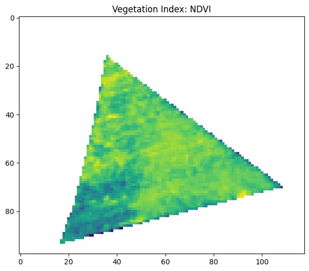
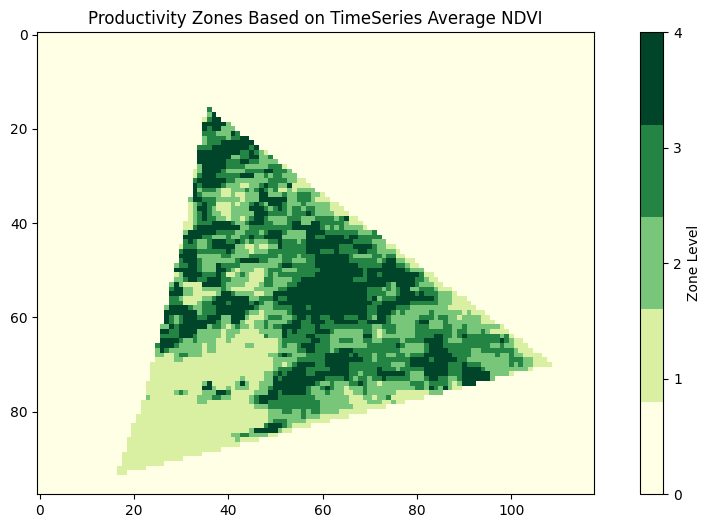
- Automatic productivity zoning from temporal NDVI composites
- Detection of regions growing differently from the rest of the field, over time
- A nitrogen proxy tracked historically, not spot-checked
- Moisture anomalies that compare a field to its own history
- Disease-risk windows derived from temperature and humidity, mapped to the field
- All of it runnable on an arbitrary polygon, with results stored and reproducible
- Index library broad enough to cover vigor, chlorophyll, water and soil-corrected variants (37+ indices implemented)
- Sentinel-2 history from January 2021 available per polygon
- Weather history joined to every index series
- One command to download, compute, and store results for a new location, with metadata and S3 paths logged
- 01
Index library
The pipeline computes NDVI, GNDVI, BNDVI, OSAVI, MSAVI, MCARI1, EVI, NDRE, NDWI, NDMI, CIRE, TVI, ARI, PSRI, NPCR, RVI, DVI, GRVI, RDVI, LAI, ExG, MWI, NDbrSMI, SCCCI, SCCCI2, CIRE2, CIRE3, MSR, MSRRE (1–3), NDVIRE (1–3), NDWI2, SAVI, SIWSI (1–2) and others. Each product picks the subset that matches its physical question rather than defaulting to NDVI.
- 02
Non-uniform growth
Regions whose index trajectory diverges from the field's are flagged. The detector runs on the series, so it catches a patch that started fine and fell behind, which a single image cannot.
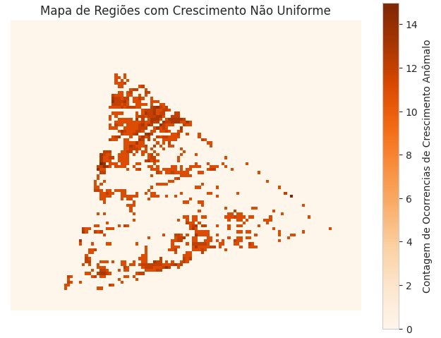
Fig. 03. Regions of non-uniform growth. Orange is where the trajectory diverged from the rest of the field. 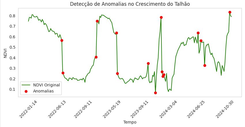
Fig. 04. The series behind the map. Red points are dates where the index moved in a way the field's history does not explain. - 03
Nitrogen from index history
Nitrogen status is estimated from chlorophyll-sensitive indices and tracked over time, per zone, so the output is a trend a fertilization plan can respond to.

Fig. 05. The field in RGB across the season, for reference. 
Fig. 06. NDVI across the same dates. 
Fig. 07. A chlorophyll-sensitive index across the same dates. 
Fig. 08. A second nitrogen-related index. Read as rows, the strips show where and when the field's nitrogen signal drifted. - 04
Moisture anomalies against the field's own baseline
The moisture product compares current NDMI/NDWI-type indices to the field's history for the same period and flags zones with humidity below expected. It also tracks which zones have been anomalous repeatedly across months.
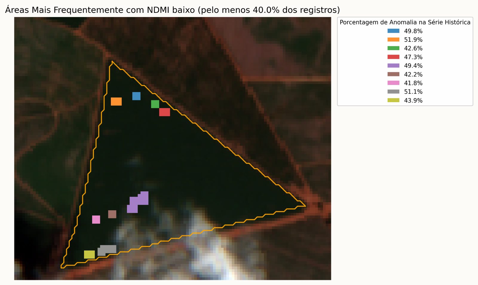
Fig. 09. Zones with a history of below-expected moisture, marked on the field. 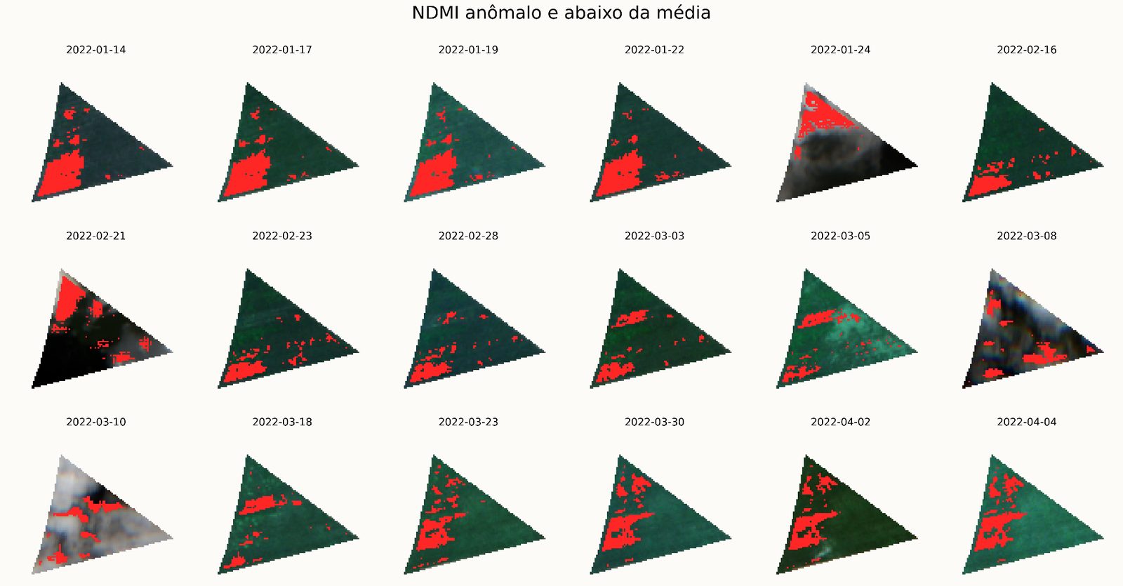
Fig. 10. Month by month: which zones were anomalous when. A zone that shows up every month is a drainage or soil issue, not weather. 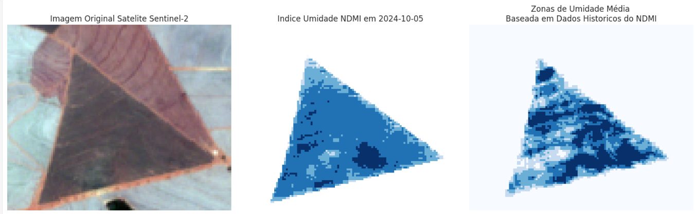
Fig. 11. RGB, NDMI, and automatic zoning of non-uniform moisture on a sugarcane field. 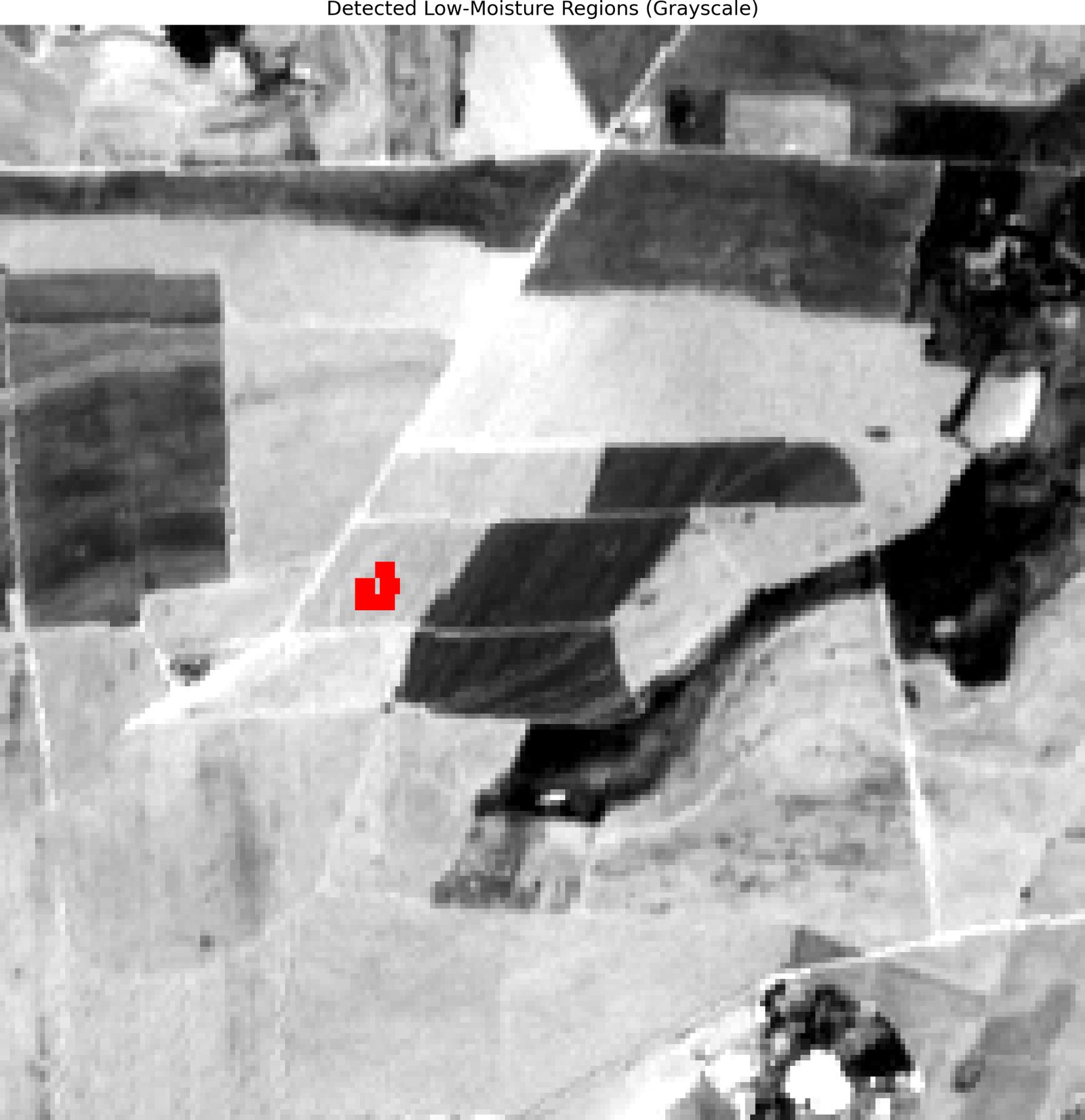
Fig. 12. Low-moisture detection now running on images containing several fields at once. Each red patch is a flagged region inside a field boundary. 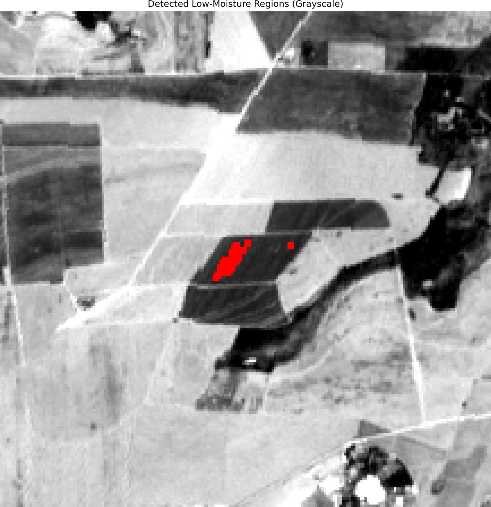
Fig. 13. Same detector, adjacent tile. 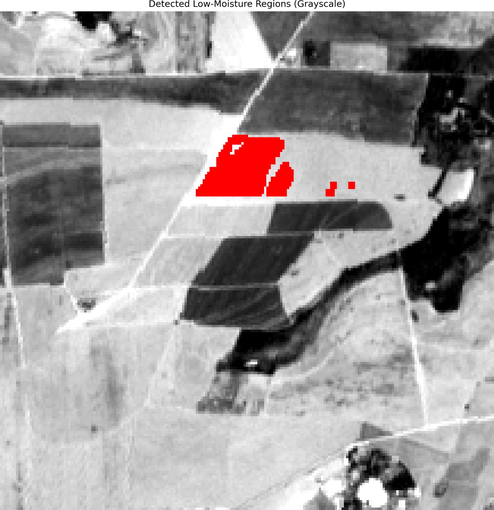
Fig. 14. Same detector, third tile. 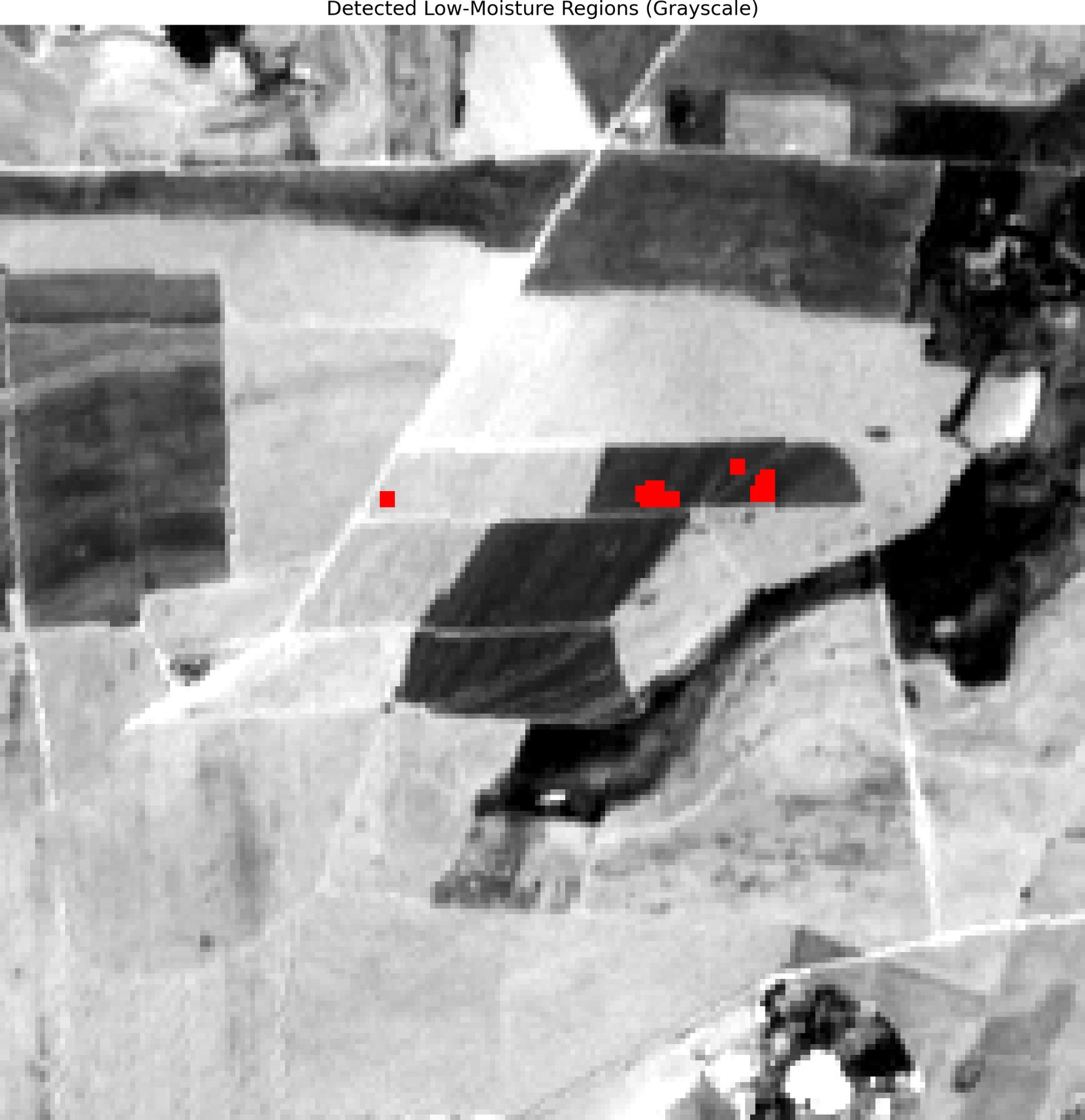
Fig. 15. Fourth tile. The first version shipped to main; classes were then refactored for the multi-field case. - 05
Disease-risk zones
Weather history is joined to the index series. Periods where temperature and humidity favor pathogen development are identified, and the field zones with the weakest vigor in those windows are flagged as risk areas.
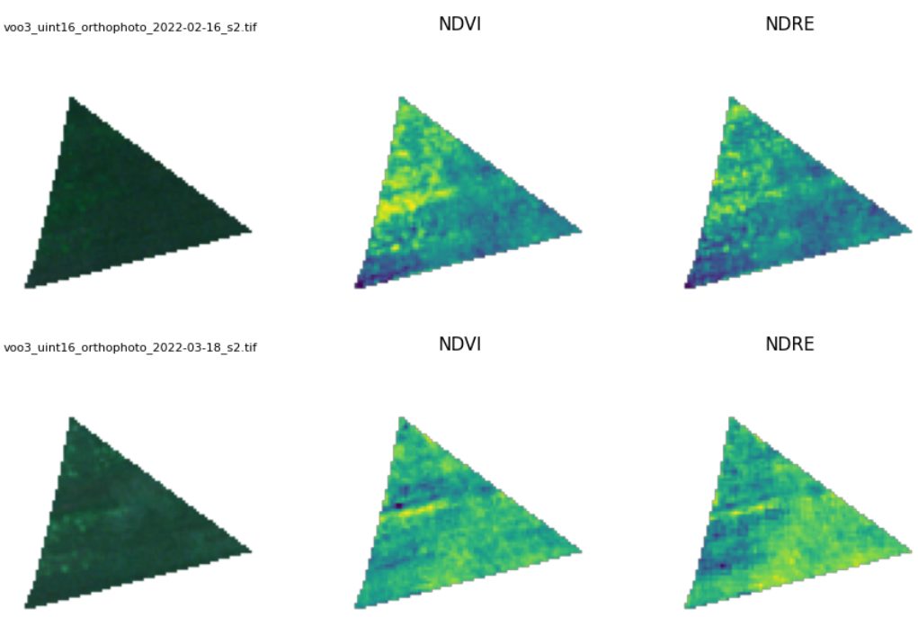
Fig. 16. NDVI and NDRE for the field across a window (16 Feb – 18 Mar 2022) where temperature and humidity favored disease. 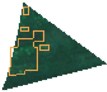
Fig. 17. The output: outlined zones to scout first, given the weather that just happened. - 06
The pipeline that runs it
All products run from one command-line tool with interactive menus, built as the simplest way to test scalability and as a demo surface for prospecting meetings. It selects a location, pulls Sentinel-2 from January 2021 onward through Google Earth Engine, stores rasters and metadata on AWS, and exposes historical index analysis, weather history, and each detector.
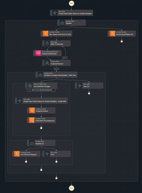
Fig. 18. The CLI: every product is a menu item. 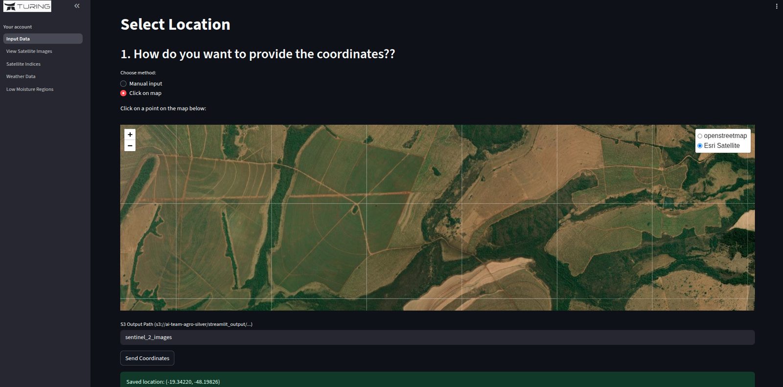
Fig. 19. Select a location: a polygon or coordinates, previewed on a map before anything downloads. 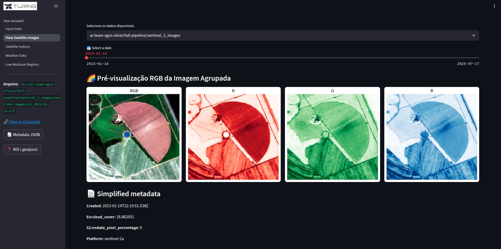
Fig. 20. Sentinel-2 history downloaded for the polygon, with band previews. 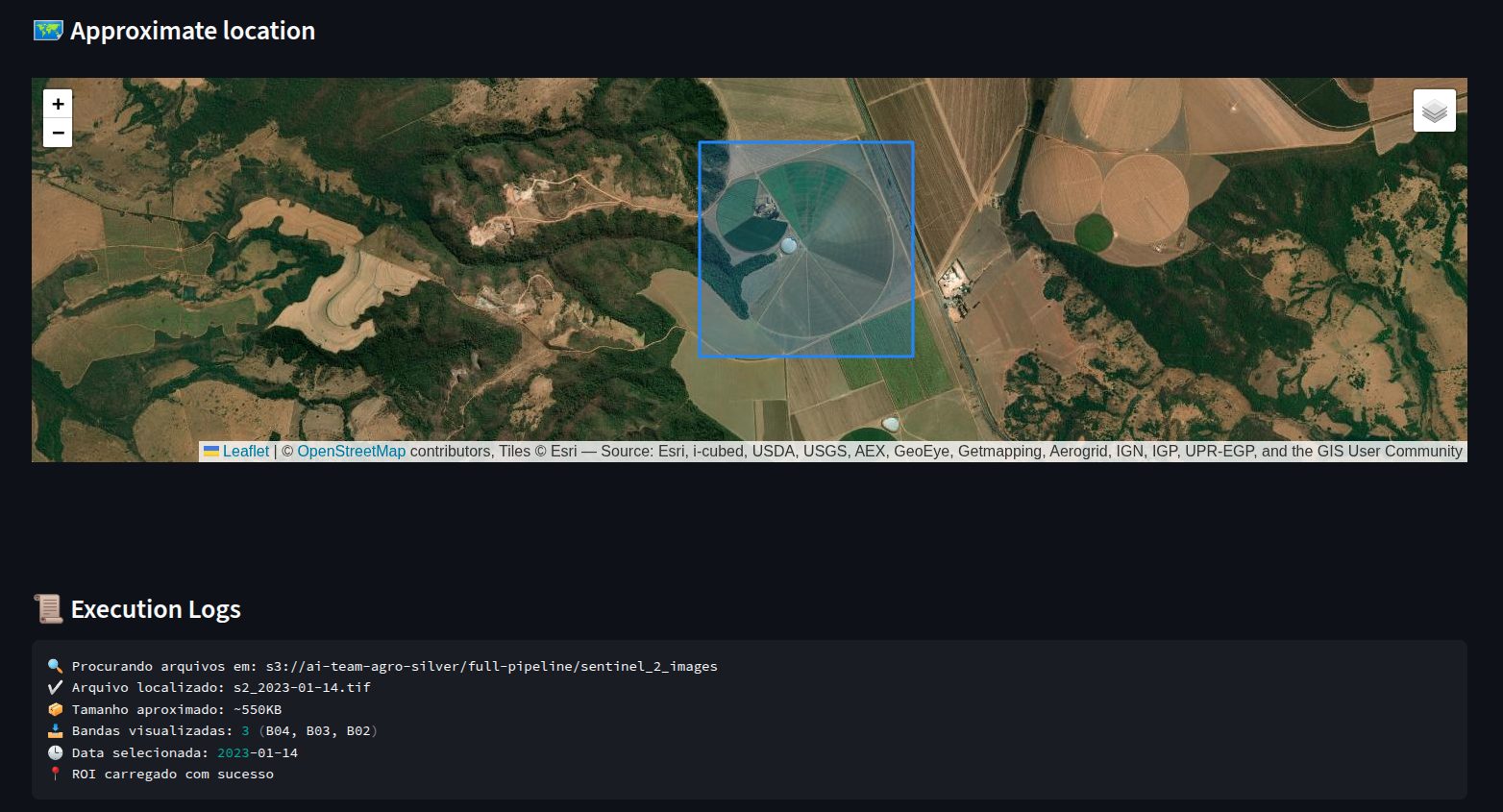
Fig. 21. Every run logs its parameters and its S3 path. Reproducible by construction. 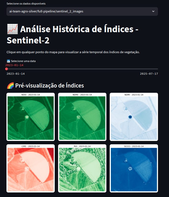
Fig. 22. Historical index analysis: choose an index, see its thumbnails over time. 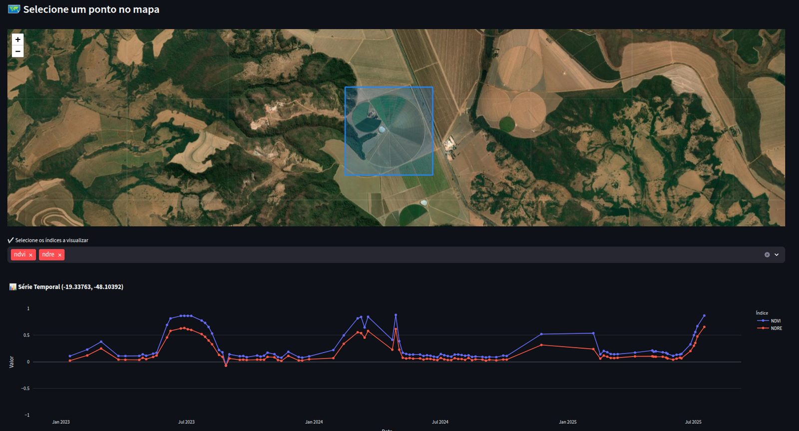
Fig. 23. The same index as a series. This is the input to every detector above. 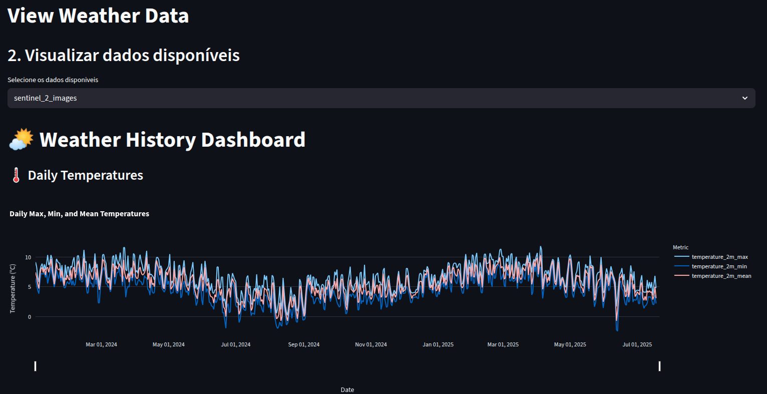
Fig. 24. Weather data for the polygon, pulled alongside the imagery. 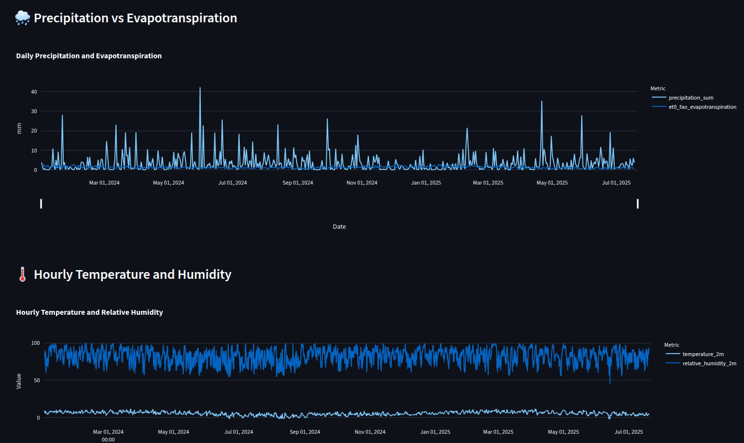
Fig. 25. Precipitation, evapotranspiration, hourly temperature and humidity: the covariates for disease risk and moisture baselines. 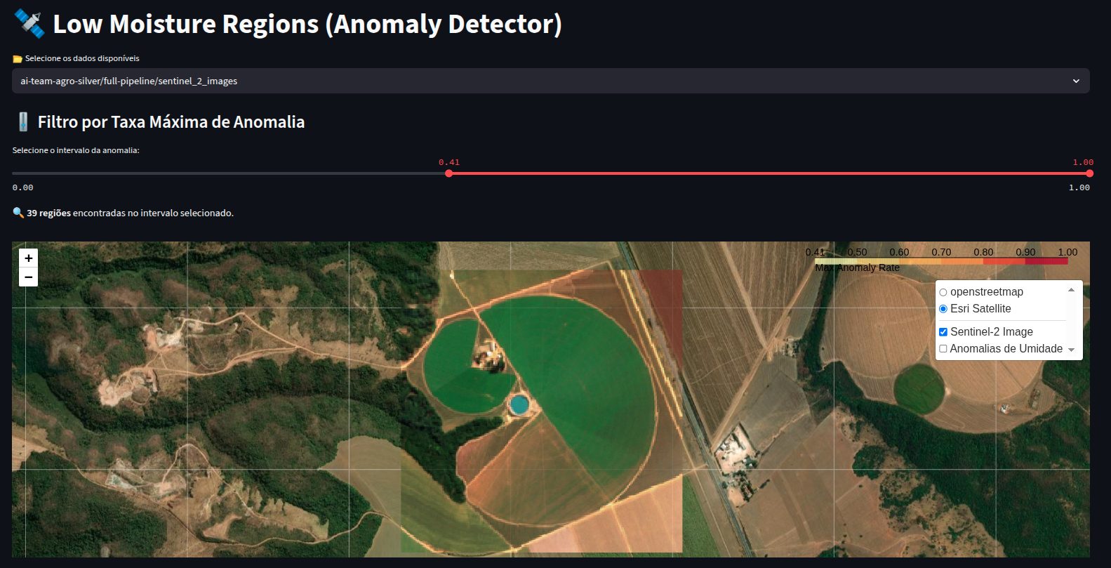
Fig. 26. The low-moisture anomaly detector running from the CLI on a chosen date. 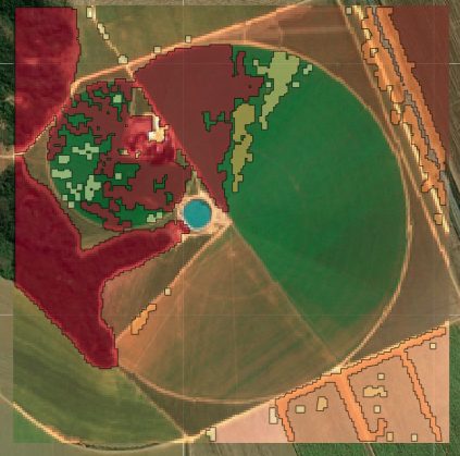
Fig. 27. Output on a property with a center pivot. The anomaly follows the pivot's coverage, which is exactly what it should do. - 07
On the roadmap
Delineate-Anything field segmentation (replacing the earlier cultivation-plot detector), disease-risk areas, crop variation analysis, best-harvest-time detection, historical harvest dates, sugarcane health analysis, a yield estimator, and temporal-series preprocessing. Each ships as one more menu item in the same pipeline.
- Temporal compositing first: every product compares a field with its own history
- A broad index library, chosen per physical question instead of defaulting to NDVI
- Weather joined at the source, so risk products are not a second system
- One CLI that doubles as scalability test and sales demo, with every run stored on S3 with metadata