Satellite imagery at 40 cm is useless for precision agriculture. Psyche AI flies the field at 4 cm across RGB, NIR, NDVI, and DVI and runs a crop-specific model that detects, outlines, and counts.
- Client
- Growers and agronomy service providers: soy, corn, sugarcane, coffee, pasture, pulp
- Industry
- Agriculture
- Problem
- Satellite imagery too coarse for per-hectare decisions
- Solution
- 4 cm multispectral capture + crop-specific detection, counting, and stress mapping
- Stack
- Drone multispectral capture (RGB · NIR · NDVI · DVI) · detection & contouring · counting · zone-level stress maps
- Live at
- psycheaerospace.com/servicos/psyche-ai
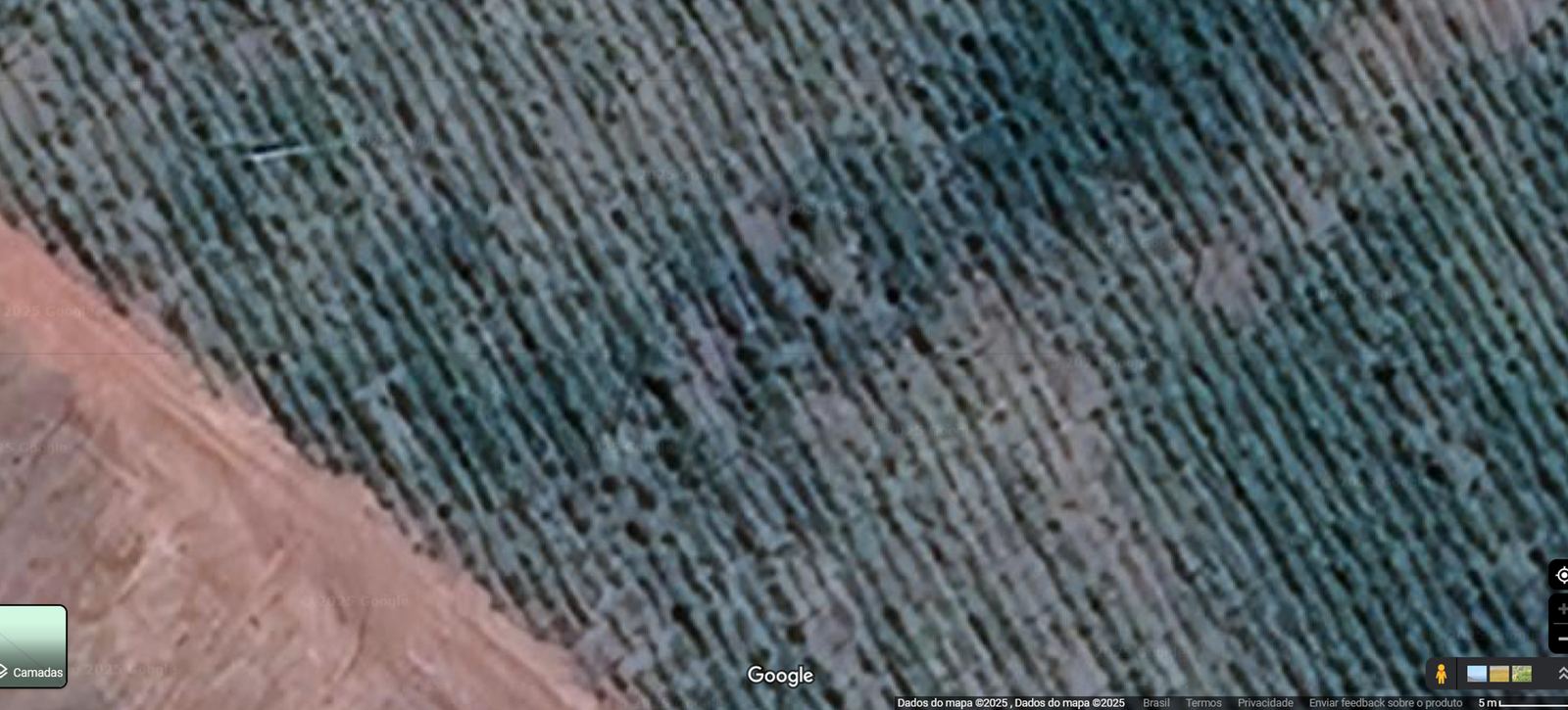
The default in crop monitoring is satellite imagery at roughly 40 cm resolution. At that scale a pest outbreak, a stand-count gap, or early disease stress does not exist. A pixel covers several plants. Growers see the problem when it is already visible from the road, then spray the whole field.
The economic gap is real and measurable: the difference between the average grower and the regional efficient frontier, in yield lost to pests, disease, and stress, plus inputs applied where they were not needed.
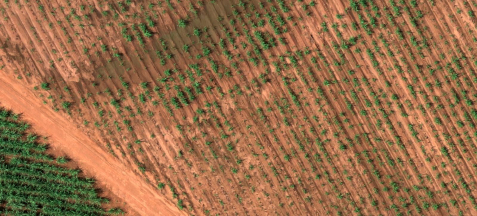
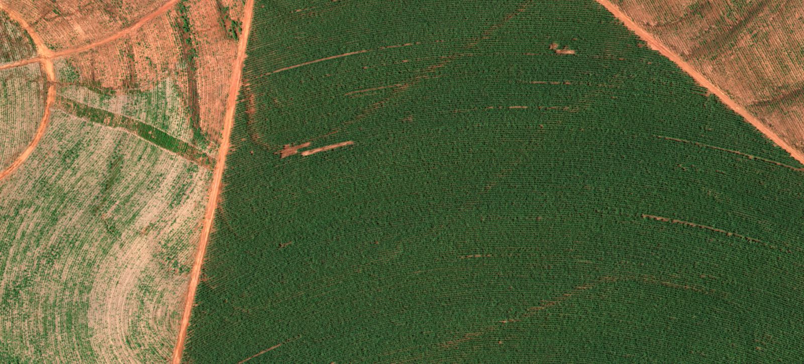
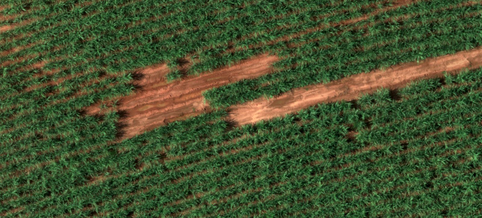
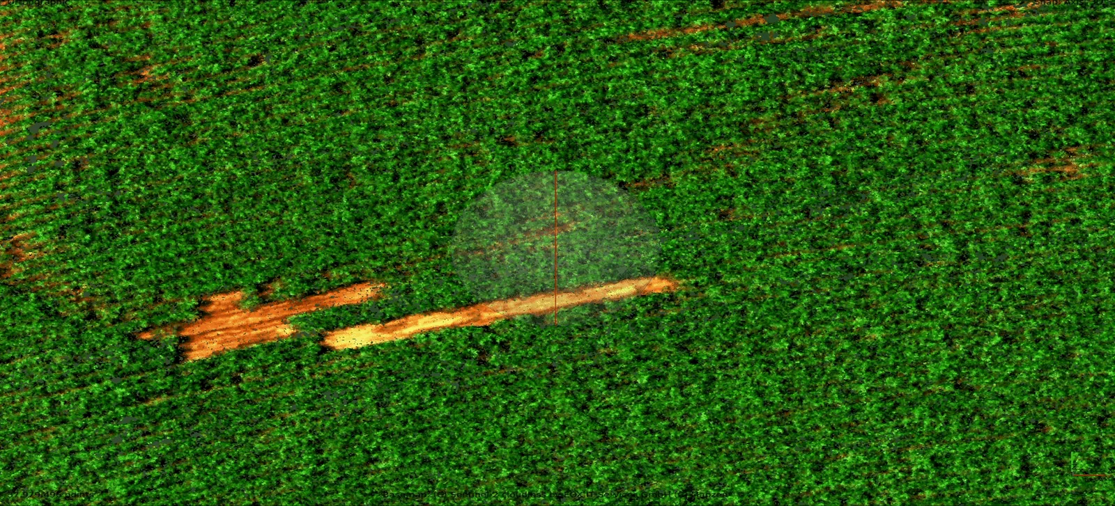
- Resolution fine enough to see an individual plant
- More than RGB: vegetation indices that expose stress before the eye can
- Crop-specific models: soy does not look like sugarcane
- An output a farm manager acts on this week, not a heatmap for the office wall
- An economic case they could defend to a CFO before committing to a season
The brief was visual. Separate the plant from the weed. Then count. Then say which hectares to walk this week.
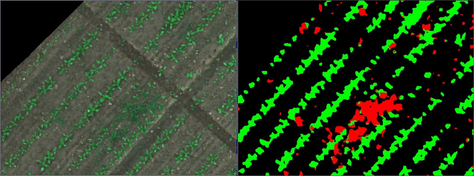
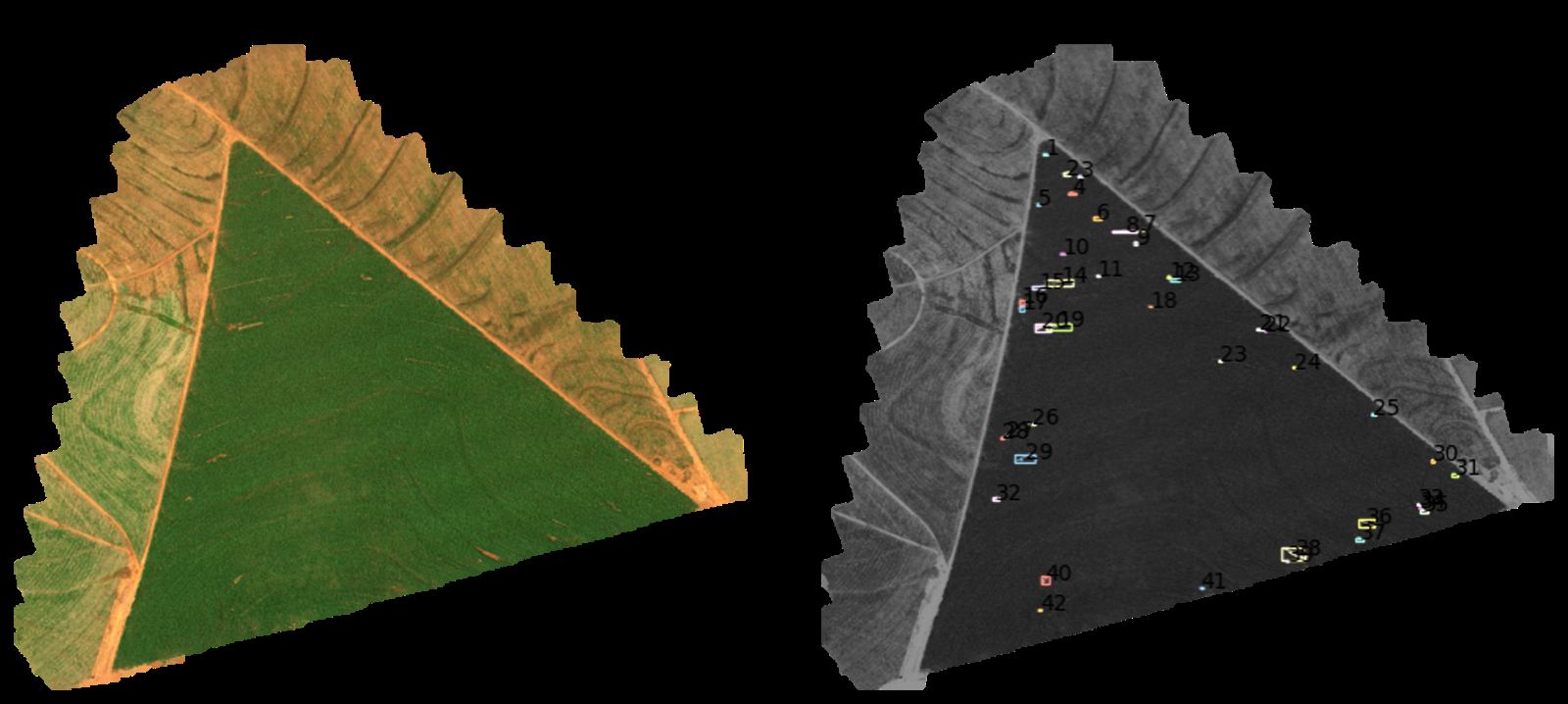
- 4 cm capture across the full property
- Plant-level detection and counting against ground truth
- Localized / variable-rate treatment instead of spraying the whole field
- 01
Capture
Drone flights at 4 cm ground resolution with a multispectral payload; the same location captured across RGB, NIR, NDVI, and DVI in a single pass.
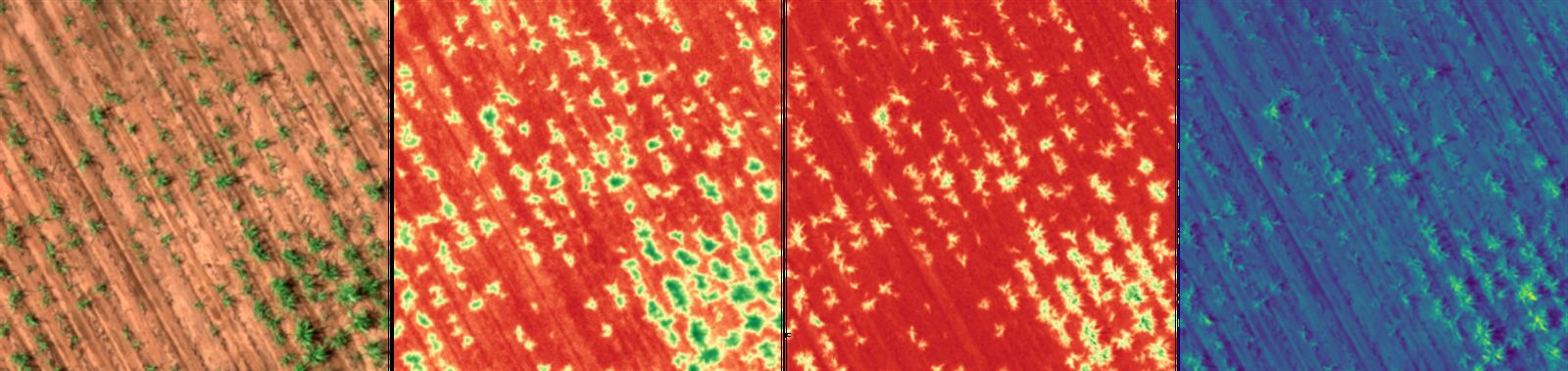
Fig. 08. One pass, four reads: natural color, vegetation index, high-contrast biomass, and a cool band for water stress. RGB is the least of it. - 02
Detection
Crop-specific models detect and contour individual plants, count stands, and map stress by zone. Each output is tied to the crop's phenological stage, because the same anomaly means different things at emergence and at flowering.
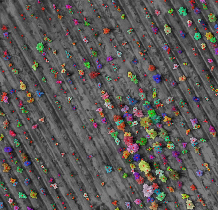
Fig. 09. Instance masks and centroids on every plant. Contour first, then count. The model is looking at organisms, not pixels. 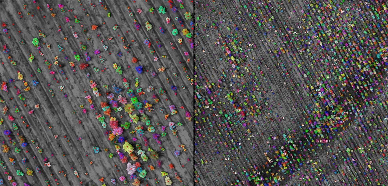
Fig. 10. The same method at two scales: a close row where each plant is a mask, and a wide pass where each plant is an ID. 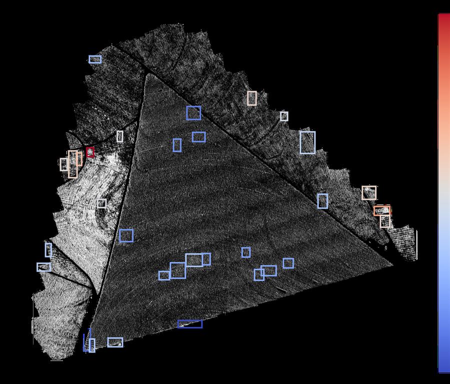
Fig. 11. Zone-level ranking on a processed scan. Color is priority, not decoration. One box at the top of the scale is the hectare to walk first. 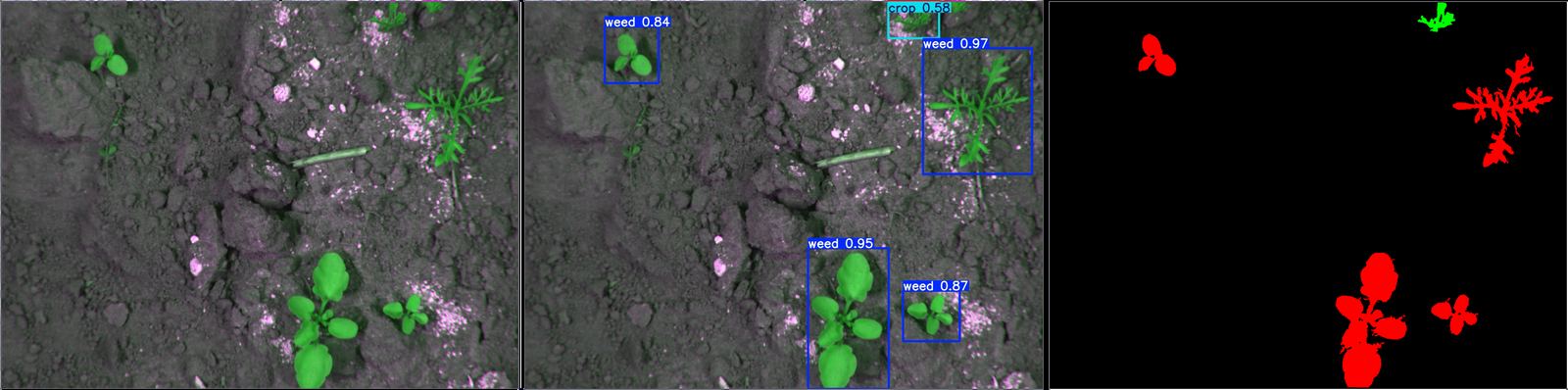
Fig. 12. Capture, classify, act. Bounding boxes name crop versus weed. The mask on the right is what a sprayer would follow. 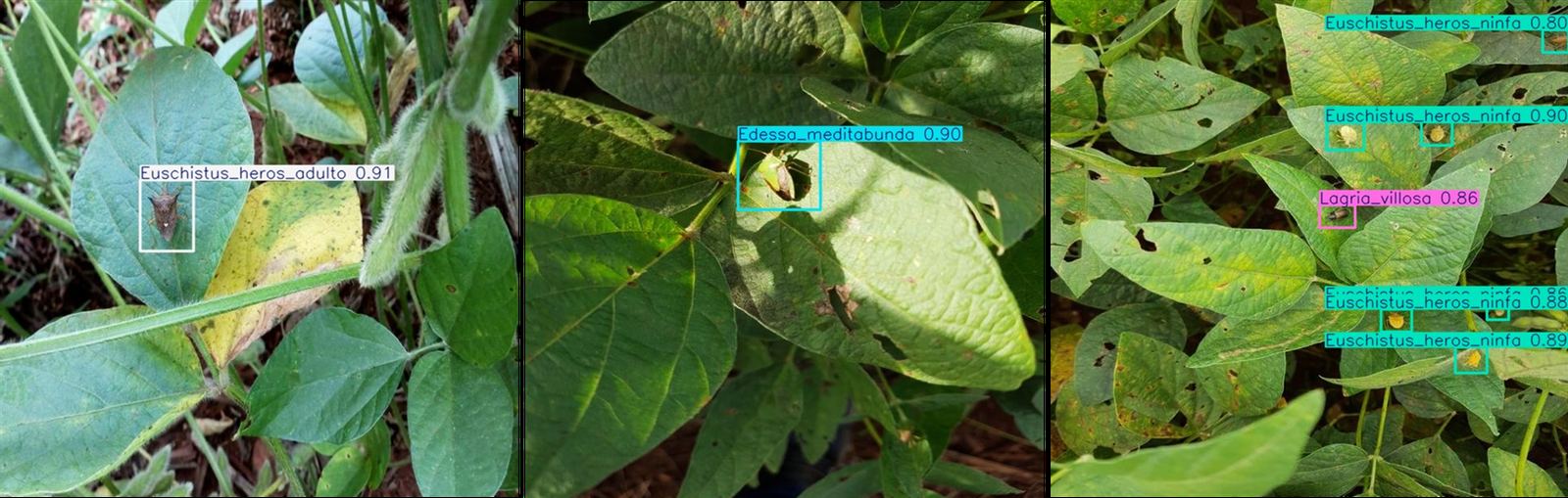
Fig. 13. Crop-specific, not generic vision. Adult and nymph of Euschistus heros, Edessa meditabunda, and Lagria villosa, each with a confidence score. - 03
Decision layer
Results are delivered as a prioritized list: which hectares, which issue, which window, rather than an image.
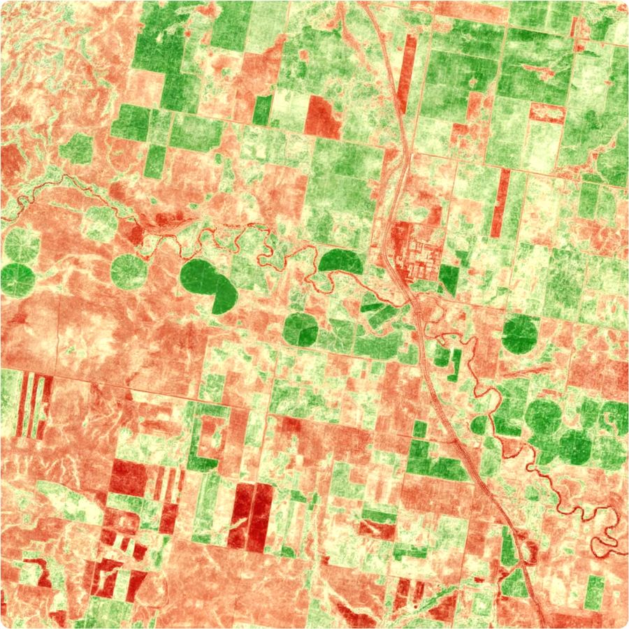
Fig. 14. A vegetation index the manager can defend in the operations meeting: which blocks are performing, which are not, at the scale of the property. - 04
Economic model
A per-crop, per-region opportunity model calibrated on public agronomic baselines (CONAB, Embrapa, regional producer data), with a ±20% confidence band declared upfront. The same model powers the public calculator on the product page.
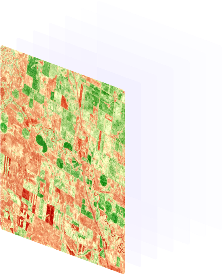
Fig. 15. The same terrain as stacked layers: spectral bands and history, not a single snapshot. This is what the opportunity model reads before it talks to a CFO.